Before we jump into the article, let's see if the conversation below sounds familiar to you anyway!

Joe: "I am the A/B testing mastermind! The green button generated 50% more clicks than the red button. My genius knows no bounds."

'Significant' Joe: "But Joe, have you considered statistical significance? I mean, we need to make sure that the difference is not just due to chance."

Joe: "Statistical significance? That's just a mean way of saying 'I don't trust your gut feeling, Joe.' But I know what I'm doing, trust me."

Months later...

'Significant' Joe: "Joe, our conversion rates haven't improved since we changed the button colour. Maybe we should reconsider our decision."

'Other' Joe: "Actually, Joe, the difference in clicks between the two buttons is not statistically significant."

Joe: "Not statistically significant? That's just mean! But seriously, guys, we should trust statistical significance from now on. After all, it's not just about being mean, it's about being statistically mean-ingful."

'Significant' Joe: "Nice pun, Joe. Maybe there's hope for you yet."

'Other' Joe: "Yeah, because let's face it, blindly trusting your gut feeling is just statistically mean-ingless."

We all have been in this situation where we are in the rush to see our hypothesis being validated while we imagine ourselves being carried on a pedestal by our colleagues and the angels from heaven feeding us grapes. This whole situation is primarily being driven by two forces - "Confirmation Bias" and "Ikea Effect"

"Confirmation Bias" is the cognitive bias where individuals selectively interpret or favour statistics that align with their preconceived beliefs, while disregarding conflicting data, enabling the ability to lie with numbers.

The "Ikea Effect" refers to the tendency for individuals to overvalue statistics or data they have manipulated or assembled themselves.

When combined, confirmation bias and the Ikea effect can be used to deceive by presenting misleading statistics that reinforce a desired narrative.

Hence its always suggested referring the "statistical significance" of these measures to rely on more objective signals. Also, that is what happens, whenever these results are in, someone from the corner of the room will just interrupt and say "Are these results statistically significant?" The whole room turns towards that voice in shock while the person fades away in the mist leaving behind just a "mic drop" moment. The same happened to me and I knew at that moment that I need to learn how to do this.

Down the line, I understood you don't need to know more than some elementary statistics to understand the roots behind this - and that's what we'll try and understand again.

Going back to the basics...

You cannot talk about statistics and not bring up the 3M's and Dispersion.

• Mean: The average value of a set of numbers, obtained by summing all the values and dividing by the total number of values.

• Median: The middle value in a sorted sequence of numbers, dividing the data into two equal halves.

• Dispersion: The spread or variability of data points around a central value.

There is one more member of this family who will be central to all our discussions going further - it's "normal" to discuss about it any discussion around statistics.

The normal curve, also known as the Gaussian distribution or bell curve, is a fundamental concept in statistics that describes a symmetrical probability distribution. The area under the normal curve holds significant meaning and provides valuable insights. The total area under the curve is equal to 1, representing the total probability of all possible outcomes.

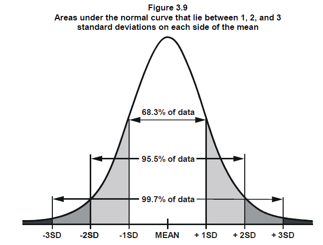
Additionally, the normal curve is characterized by its empirical rule, which states that approximately 68% of the data falls within one standard deviation of the mean, 95% falls within two standard deviations, and 99.7% falls within three standard deviations. Thus, the area under the normal curve provides valuable information about the likelihood and distribution of data points.

The normal curve is so humble that it named itself "normal." Despite being the go-to distribution for many statistical analyses, it decided to go with a simple and unpretentious name, perfectly capturing its modesty. It truly exemplifies the saying, "I'm not special, I'm just normal...ly distributed!"

What's an A/B Test?

An A/B test, also known as a split test, is a statistical technique used to compare two versions of a variable or treatment. Its true essence lies in comparing an experiment situation (Group A) with a control situation (Group B). The purpose is to evaluate the impact of the changes introduced in the experiment situation by comparing it to the control situation. The difference in the value of the metric we are measuring in these situations is what needs to be "statistically significant".

That's the pitfall many people generally fall for is the face value of this delta/difference - just because it's high won't translate into whether it's significant or not. Don't worry if you don't get this part, we'll come back to this down the line.

Some statistical chops...

To further go on with our discussion we need to understand some more theorems. Feel free to use these in discussions with your peers and enjoy some "mic drops" moments.

Central Limit Theorem

The Central Limit Theorem states that as the sample size increases, the sampling distribution of the mean (or sum) of independent and identically distributed random variables will become approximately normally distributed, regardless of the shape of the population distribution.

This means that even if the individual observations are not normally distributed, the distribution of the sample mean will tend towards a normal distribution as the sample size increases.

This is a critical part to understand so let's deep dive into this and understand this with an example.

Let's say, you have a population of 1000 individuals, and you're interested in their heights. You take random samples of 100 students from this population multiple times, and for each sample, you calculate the mean height. Let's call the means from each sample M1, M2, M3, and so on.

According to the Central Limit Theorem, as you repeat this process and collect more and more samples, the distribution of these sample means (M1, M2, M3, and so on) will tend towards a normal distribution. This normal distribution of the sample means is crucial because it allows you to make statistical inferences, such as calculating confidence intervals or performing hypothesis tests, even if the original population distribution (heights of 1000 students) is not normally distributed.

We can derive many conclusions basis this theorem - Let's say we take two sample memes from this distribution, M1 and M2. Let's say the difference between these two values is D1 so, D1 = M1 - M2. Now since the means are normally distributed we can derive conclusions like,

Now, based on the properties of the normal distribution, we can derive conclusions by examining the difference D1 in relation to the standard error (SE) of the distribution.

We'll further explain how you can calculate the SE while running the experiment. For now, let us assume we know it beforehand.

Let's say the standard error is 10 (just for illustration purposes). In this case, if the difference D1 is less than or equal to 1 standard error (1 SE) of the distribution, we can make the following conclusion:

If D1 <= 1 SE of the distribution, the chances that these means came from the same population is approximately 68%.

This conclusion is based on the fact that approximately 68% of the values in a normal distribution fall within 1 standard deviation (1 SE) from the mean. (refer to the diagram we showed at the top) So, if the difference D1 is within this range, it suggests that the two sample means are not significantly different from each other, and it is likely that they are from the same population.

Coming back to A/B Testing

To be honest, we have already explained the science behind A/B testing. At its core, significance testing aims to answer a fundamental question:

What is the probability that the observed differences between two samples are simply a result of random variation?

To address this question, we measure the extent of the distance between the sample values, quantified in terms of standard errors (SE). In significance testing, we often express the difference between sample means in terms of standard errors, such as 1SE or 2SE. The magnitude of the difference, measured in terms of standard errors, provides valuable insights into the likelihood that the two samples come from the same population.

Let's wrap this up with a relatable example!

Suppose you are conducting an A/B test to compare the click-through rates (CTR) of two website versions: Version A and Version B. You collect data from a random sample of 500 visitors for each version and calculate the CTR for each group.

In Version A (the control group), you observe 50 clicks out of 500 visitors, resulting in a CTR of 0.10 (10%). In Version B (the experiment group), you observe 75 clicks out of 500 visitors, resulting in a CTR of 0.15 (15%).

1. Calculate the standard error for each group:

   • The standard error for Version A (SE1):

     • SE1 = sqrt(p1 (1 - p1) / n1)

     • SE1 = sqrt(0.10 (1 - 0.10) / 500) ≈ 0.0141 (or 1.41%)

   • The standard error for Version B (SE2):

     • SE2 = sqrt(p2 (1 - p2) / n2)

     • SE2 = sqrt(0.15 (1 - 0.15) / 500) ≈ 0.0162 (or 1.62%)

1. Calculate the SE-diff:

   • SE-diff = sqrt(SE1^2 + SE2^2)

   • SE-diff = sqrt((0.0141)^2 + (0.0162)^2) ≈ 0.021 (or 2.1%)

1. Assess the statistical significance: To determine the statistical significance, you can compare the observed difference in CTR (0.15 - 0.10 = 0.05 or 5%) with the SE-diff.

If the observed difference is greater than or equal to 2 times the SE-diff (i.e., 2 * 0.021 = 0.042 or 4.2%), we can conclude that the difference is statistically significant at a desired level of confidence (e.g., 95%). You can refer to the diagram to understand why 2 times SE-diff.

In our example, the observed difference (5%) is larger than 2 times the SE-diff (4.2%), indicating that the difference in CTR between Version A and Version B is statistically significant at a desired level of confidence.

By calculating the standard error from samples and then using the SE-diff, we can assess the statistical significance of the A/B test results. This allows us to make informed decisions about whether the observed difference between the groups is likely due to the tested changes or if it could be due to random chance.

Why do pitfalls happen?

Now that we understand the science behind A/B testing we can also reason why we cannot take the difference between our samples at face value. We observed that SE is directly proportionate to SD of the sample coz, SE = SD / sqrt(n) . We also observe that SE-diff is directly proportional to SE which does imply that SE-diff is directly proportional to SD.

Thus if we take on the difference between control and experiment only on face value. Let's say the marks of students taking a test in two different situations (lets say we are testing the effect of some mind-enhancing drug) has a mean difference of 30 marks. We might be inclined to agree on the increase of the marks - but if the underlying standard deviation is high then we'll need a way bigger gap in marks to have at least 2 times SE-diff for a 95% acceptance. Thus doing a significance test always comes in handy.

Some other supporting metrics

We don't really need to stop at just significance testing to support our A/B experiments. There are a bunch of other analyses that you could do - to make your assessment more comprehensive.

Metrics’ Delta Confidence Interval

Confidence interval contains richer information than single significant status. Using confidence intervals, we can evaluate the expected range of lift (or decline) of the considered metrics.

Let's assume the metrics’ delta confidence interval is 1.89% — 3.27%, meaning we would get a metrics lift of 1.89% — 3.27% if we roll out the revamped design into production (i.e., we win the variant group).

Experiment’s Statistical Power

Statistical power is the ability of the experiment to detect an effect (metrics difference) that is actually present in reality (the ground truth).

Let's assume the statistical power of the experiment is 54.8%. That is, the likelihood is 54.8% for the experiment to detect a non-zero effect (i.e., change between variant and control is different) if there is truly an effect in reality.

I found a pretty comprehensive article which dives into how you can calculate the above two supporting metrics.

Concluding Thoughts

When diving into the fascinating world of statistics, it's important to remember that it's like a quirky, directional entity. And when it comes to A/B testing, let's not get too carried away with it!

Sure, statistical analysis gives us some cool insights into the differences between samples. We love comparing Version A and Version B to see which one rocks. But here's the thing: stats is just one part of the story.

In A/B testing, it's easy to get fixated on finding that "winning" version or obsessing over statistical significance. But let's not forget the bigger picture, folks. We need to consider user experience, context, and practical significance alongside our trusty statistical tools.

Think of it this way: stats is like a trusty sidekick, but it's not the superhero saving the day all on its own. We've got to bring in other factors and use some good old common sense too. A holistic approach to A/B testing involves considering various factors, such as user experience, context, and practical significance, alongside statistical analysis.

Some other gotcha's

1. Depending on sample size we can also either do a t-test or a z-test to go onto the journey of statistical significance.

2. There are other cases of One-Tailed vs Two-Tailed tests in A/B testing

   1. One-Tailed Test: A one-tailed test in A/B testing focuses on detecting differences in a specific direction. It examines whether one sample is significantly greater or smaller than the other sample, based on a directional hypothesis. It is used when we have a clear expectation or hypothesis about the direction of the difference between the samples.

   2. Two-Tailed Test: A two-tailed test in A/B testing assesses whether there is a significant difference between the samples, regardless of the direction. It allows for the detection of differences in either direction and is commonly used when there is no specific expectation about the direction of the difference.

      Choosing between the two: The choice between a one-tailed and a two-tailed test depends on the research question and prior knowledge. A one-tailed test is more sensitive to detect differences in a specific direction, while a two-tailed test provides a broader assessment of any significant difference between the samples, regardless of direction.

   3. The chi-squared test is commonly used in A/B testing when we are comparing categorical variables or proportions between two or more groups. It helps us determine if there is a significant difference in the distribution of categorical data across the groups being compared.

   4. The F-test is commonly used in statistical analysis to compare the variances of two or more groups or to assess the overall significance of a regression model.

Resources

1. I read the book "Statistics without Tears"

2. Also an article on how to make your A/B test more comprehensive.